Terminated Transmission Lines

This case study looks into a regular transmission line simulation and the effects of differently matched loads on the wave propagation. Here, the transmission line is of a simple form and is represented as a pair of metallic planes, where the Gaussian pulse, input at one end, propagates to the other, loaded with different materials of specific impedance values (Fig.1a). These, in turn, define the reflection coefficient ( $\Gamma$ ) and, hence, subsequent impulse behavior. For a transmission line with the characteristic impedance $Z_0$ terminated with a load of impedance $Z_L$ , the reflection coefficient is defined as

(1) $\begin{equation*}$\Gamma$ = ${Z_L - Z_0} \over {Z_L + Z_0}$\end{equation*}$

Let’s take a look at three special load cases [1].

1. Matched load case ( $Z_L=Z_0$ ).

When the load impedance matches the characteristic one, the reflection coefficient turns zero and the pulse passes completely through the load. To create such a matched load on MaxLLG, a brick of dielectric conductivity should be added between the metallic planes at their end (Fig.1a (upper)). The exact value should be evaluated through the following steps:

Run the simulation with an arbitrary conductivity value to find the characteristic impedance. Take into account the signal load value and the signal amplitude set in the metascript. Here, they’re equal to 50 Ohm and 1 V/m, respectively. Looking at the output files, the resulting pulse amplitude indicates an impedance ratio, since the line acts as a voltage divider. For example, in the simulation provided, the voltage on the line is the electric field between the planes (32.5 kV/m) times the distance (20 um) which results in 0.65 V and, consequently, in the line resistance being 92.86 Ohm.
Next, calculate the resistivity by multiplying the resistance (92.86 Ohm) by the load cross-section area (200 um²) and dividing by its length (4 um). The reciprocal of the resistivity value (4.6 mOhm•m) gives the required load conductivity (215.4 S/m).

Fig.1b (upper) and Fig.1c illustrate the simulation results that correlate with the calculations above.

2. Short-circuit load case ( $Z_L=0$ ).

When the transmission line is terminated with a metallic wall (Fig.1a (middle)), $\Gamma$ =-1 and the signal is completely reflected with a phase switch to the opposite. This effect can easily be seen in Fig.1b (middle) and Fig.1d.

3. Open circuit load case ( $Z_L \rightarrow \infty$ ).

Finally, when the line is open-ended (Fig. 1a (lower)), the load impedance significantly exceeds $Z_0$ , so that $\Gamma$ =1 and the pulse is reflected without any changes (Fig.1b (lower) and Fig.1e).

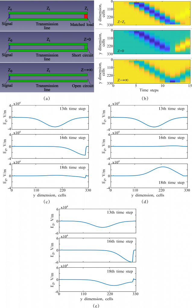
Fig. 1 (a) Transmission lines terminated with differently matched loads; (b) Time maps of the signal propagation in the transmission lines; (c-e) Electric field profiles in the lines terminated with matched load (c), short-circuit load (d), and open-circuit load (e) at several time steps.

[1] Pozar D.M., Microwave Engineering, John Wiley & Sons, Inc., 2011.

To recreate the figures above, one can utilise the following Matlab code:

%TIME MAP (Fig.1b)
IE=30; %number of cells in x-direction
JE=330; %number of cells in y-direction

firstnumber=5; %number of a time step to begin with
lastnumber=19; %number of a time step to end with
NFRAMES=lastnumber-firstnumber+1;
figure
axis tight
w_k=ones(JE,NFRAMES);
jj=0;
for k=firstnumber:lastnumber
    jj=jj+1;
filename = ['out_xy.',num2str(k,'%d')]; %read the output data from the each file 
a=load(filename); 

n=0;
for j=1:JE 
    for i=1:IE
        n=n+1;
        b(j,i)=a(n,1); %set the proper field component column (here, 1 stands for e_z) 
    end
end

w_k(:,jj)=b(:,15); %collect all field values across a x-coordinate for a given frame 
jj

end

%MOVIE AND FIELD PROFILE (Fig.1c-e)
IE=30; %number of cells in x-direction
JE=330; %number of cells in y-direction
b=ones(JE,IE);
firstnumber=0; %number of a time step to begin with
lastnumber=19; %number of a time step to end with
figure
axis tight

jj=0;
for k=firstnumber:lastnumber
    jj=jj+1;
filename = ['out_xy.',num2str(k,'%d')]; %read the output data from the each
a=load(filename);

n=0;
for j=1:JE
    for i=1:IE
        n=n+1;
        b(j,i)=a(n,1); %set the proper field component column (here, 1 stands for e_z)    
    end
end
Ez(:,jj) = b(:,15); %collect all field values across a x-coordinate for a given frame
subplot(2,1,1)
imagesc(b); %display the pulse heatmap in xy-plane
subplot(2,1,2)
plot(Ez(:,jj)); %display the field profile
axis([1 350 -4e4 4e4])
drawnow
pause(0.5e-0);
jj
end

Terminated Transmission Lines

You May Also Like

Magnetic Patch Antenna

Leave a comment Cancel reply