Dispersion characteristics for a magnetostatic wave in tangentially magnetized medium placed inside a parallel plate waveguide

In this example we show the dispersion characteristic obtained for a backward volume magnetostatic wave (BVMW) propagating in magnetic dielectric medium placed inside a parallel plate waveguide. The numerical solution is produced by MaxLLG and compared with the analytical formulation derived for a linearised solution of LLG equation [1] along with Maxwell equations. The wave is linearly polarised and propagates in the direction parallel to the magnetic field $H$ and magnetisation $M$ (aligned with axis $y$ ). The electric conductivity of the medium $\sigma$ is zero and the relative permittivity $\varepsilon_r$ is constant. The analytical dispersion relation is

(1) $\begin{equation*}-k^2_z[\mu k^2_z + (1+\mu)k^2 - (\mu^2 + \mu - \mu_a^2)k^2_0 \varepsilon_r] = k^4 - 2\mu k^2 k^2_0 \varepsilon_r + (\mu^2 - \mu^2_a)k^4_0 \varepsilon^2_r,\end{equation*}$

where $\mu$ and $\mu_a$ are diagonal and off-diagonal (gyrotropic) components of the permeability tenzor, $\omega_H = \gamma H$ is the resonance frequency, $H$ is the applied magnetic field, $\omega_M = 4 \pi \gamma M_0$ , $4 \pi \gamma M_0$ is the saturation magnetization, $\gamma$ is the gyromagnetic ratio, $k$ is a wavenumber in the y direction, $k_0 = \omega/c$ is the wavenumber of EM wave propagating in vacuum, $\omega = 2 \pi f$ is a circular frequency, $k_z$ is the frequency-dependent function [2] and can be written using the magnetostatic approximation as

(2) $\begin{equation*}k_z = n \pi / d,\end{equation*}$

$n=\pm 1, 2, 3,..$ is an arbitrary integer corresponding to a wave mode, $d$ is a layer thickness. Thus, the dispersion relation can be rewritten as:

(3) $\begin{equation*}$\varepsilon_r^2 \omega^6 - \omega^4 [\varepsilon_r^2 (\omega_H + \omega_M)^2 - 2 c^2 \varepsilon_r (k^2+k_z^2)] + \omega^2 \{ c^4 (k^2 + k_z^2)^2 + c^2 \varepsilon_r (\omega_H + \omega_M) \cdot \\ \cdot [2k^2 \omega_H + k_z^2(2\omega_H + \omega_M)]\} - c^4 (k^2 + k_z^2) \omega_H [k^2 \omega_H + k_z^2(\omega_H + \omega_M)] = 0$.\end{equation*}$

The equation (3) is based on the linearised solution of Landau-Lifshits-Gilbert equation [1] with the dispersion curve shown on Fig. 1d. Note, this equation does not allow for an explicit functional relation but a numerical formulation (to any degree of precision) can be easily done (Fig. 1d red line).

As in other case studies, the first step in simulating the dispersion of the waves propagating in the unbounded ferrite is to create an input file of the media. In case of long structures having the same cross-sections it is easier to use 2D formulation. For this purpose one can upload a png image of the model cross-section to the 2D Image Files section (make sure to avoid anti-aliasing effects normally present in all modern graphic editors. Each colour should represent only one particular material) The picture made for the given example is shown in Fig. 1a. All sizes are set in pixels (px) and the picture shows three regions corresponding to different materials: ferrite (green square), metal (red rectangles) and air (blue area). The latter is necessary to include the periodic boundary condition (PBC) or Perfectly Matched Layer (PML) which are needed to either replicate the given geometry to an infinite extent or use absorbing layers accordingly. In this particular example we use the following dimensions and parameters given in Fig. 1a and Fig. 1b accordingly. Once the matrix file is created, the next step is to set parameters in the metascript file. In this case the medium was excited with the magnetic field pulse located in $y$ = 500, all cell sizes were 0.2 mm so the layer thickness $d$ was 1 mm, and the applied field was aligned with axis $y$ . To have ferrite unbounded in a propagation plane PBC were set for $x$ – and $y$ -directions. Along $z$ -axis there were PML conditions implemented outside the plates.

During simulation MaxLLG takes field intensity maps in the medium planes every Nth frame, where N is set at the Parameters step (Fig. 1c). Here, an x-component of the magnetization is considered. When the simulation is complete, an array of field profiles along y axis at fixed point $x_0$ for each frame is taken and combined chronologically in a new space-time map (only for one particular orientation where profiles are collected – this is the orientation of the sought dispersion). So a time map is made where the field evolution in the structure is seen (inclusion in Fig. 1c). The Fig. 1d demonstrates the results of the two-dimensional Fourier transform of the space-time map compared with the analytical ones obtained using (1-2). One can see that dispersion curve of the BVMW first mode (a red line) correlate very well with the numerical solution (yellow dots) with the exception of the cutoff. Thus, according to the analytical theory the BVMW’s cutoff is the ferromagnetic resonance frequency of perpendicularly magnetized ferrite , while the simulation shows its absence. This discrepancy may be of the coupling effect, when the magnetostatic wave interacts with the fast electromagnetic one, that is not taken into account in the theory.

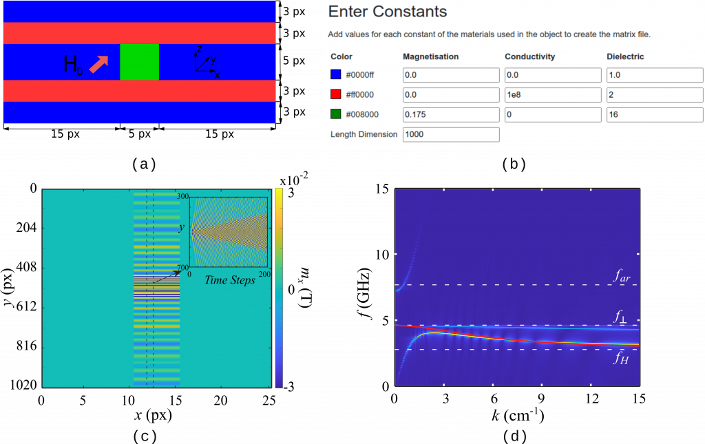
Fig. 1. a) Image of the model cross-section showing two regions corresponding to different materials: ferrite (green square), metallic plates (red rectangles), and air (blue area). b) Medium parameters used in the simulation. c) A field intensity map taken in x-y plane, and a space-time map collected of field profiles at point $x_0 = 12$ px (inclusion). d) The dispersion characteristic obtained for a plane electromagnetic wave propagating in tangentially magnetized medium placed inside a parallel plate waveguide by means of MaxLLG (yellow points) and the analytical formulation (red lines) with parameters: $4 \pi M _s=1.75$ kOe, $H=1$ kOe, $\alpha=0.001$ , $\varepsilon _r =16$ .

[1] Gurevich A.G., Melkov G.A., Magnetization Oscillations and Waves. CRC Press, Inc; 1996. 445 p.
[2] Mikaelyan A.L., Theory and practice of microwave ferrites. State Power Press, Moscow; 1963. 663 p. (in Russian)

Dispersion characteristics for a magnetostatic wave in tangentially magnetized medium placed inside a parallel plate waveguide

You May Also Like

Dispersion characteristics for a magnetostatic wave in unbounded medium

Faraday rotation

Leave a comment Cancel reply