Faraday rotation

In this example we compare the results of our model with the analytical solution for a plane electromagnetic wave propagating in magnetic dielectric medium. The wave is linearly polarised and propagates in the direction of the constant applied magnetic field H (aligned with axis y). The electric conductivity of the medium $\sigma$ is zero and the relative permittivity $\epsilon _r$ is constant. The analytical solution for the electric field as a function of spatial variable can be described as follows [1]:

(1) $\begin{equation*} $\overline{E} = E_0 \Large{ \textnormal{[}} \hat{z} \normalsize \textnormal{cos} \huge \textnormal{(} \dfrac{\beta _+ - \beta _-}{2} \huge \textnormal{)} y - \normalsize \hat{x} \textnormal{sin} \huge{(}\dfrac{\beta _+ - \beta _-}{2} \huge \textnormal{)}y \huge{ \textnormal{]}} e^{-i (\beta _+ + \beta _-) y/2} $ \end{equation*}$

where $\beta _{\pm} = \omega \sqrt{\epsilon (\mu \pm \kappa)}$ are the propagation constants for right hand circular (subscript ‘+’) and left hand circular (subscript ‘-‘) modes, with $\mu$ and $\kappa$ being the diagonal and off-diagonal (gyrotropic) components of the permeability tensor [Pozar]. Due to different frequency dependence of the two constants, the polarisation of the electric field vector becomes a function of the spatial variable. This is especially seen close to the resonance frequency $\omega _H = \gamma H$ , where $H$ is the applied magnetic field. Depending on the damping coefficient $\alpha$ , $\beta _+$ can significantly overcome $\beta _-$ leading to faster rotation of the polarisation. The angle of rotation, as a function of the spatial variable $y$ can be then determined from:

(2) $\begin{equation*} $\phi = \textnormal{tan} ^{-1} \dfrac{E_z}{E_x} = - \huge \textnormal{(} \dfrac{\beta _+ - \beta _-}{2} \huge \textnormal{)} y$ \end{equation*}$

For frequencies below $\omega_H$ the sign of $\phi$ is negative, indicating that the rotation of polarisation is counter-clockwise (the same as for the right-hand circular mode). For higher frequencies $\phi$ changes the sign to positive. In the special case of $\omega_H < \omega < \omega _H + \omega _M$ and if no losses are present $\beta _+$ becomes purely imaginary, so only left circular mode can propagate in the media. If $\alpha$ is non-zero then RHCP mode can be present too, but only as an evanescent wave.

Results and Discussion

Figure 1 shows a field map of electric field component $E_z$ produced by MaxLLG solver for a case of a magneto-dielectric medium with parameters: $4 \pi \textnormal{M} _s=1.8$ kOe, $H=6$ kOe, $f=11$ GHz, $\alpha=0.001$ , $\epsilon _r =13$ , cell dimensions $0.25$ mm in all directions. The solution is produced for a case with Periodic Boundary Conditions (PBC) in transverse directions to propagation. The excitation of the electric field is achieved in the initial x-z plane (at pixel $15$ ) with a uniform continuous source with the above frequency.

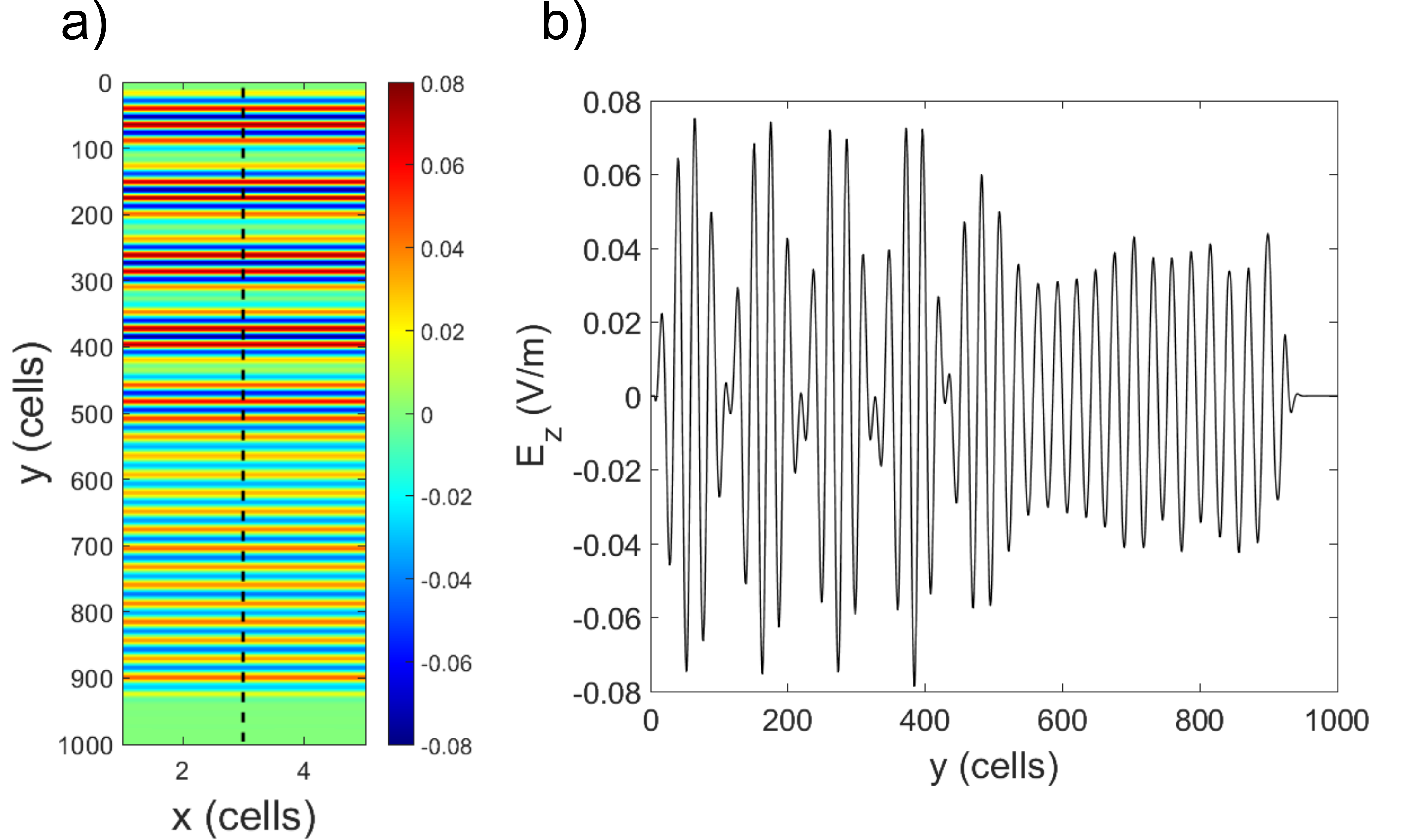
Fig. 1. a) Map of $E _z$ component produced by MaxLLG (time step $dt=7000$ from x-y plane in the middle of the grid. Blue arrows show the position of the PBC boundaries. All fields within PBC boundaries are the same, as should be for a plane wave.

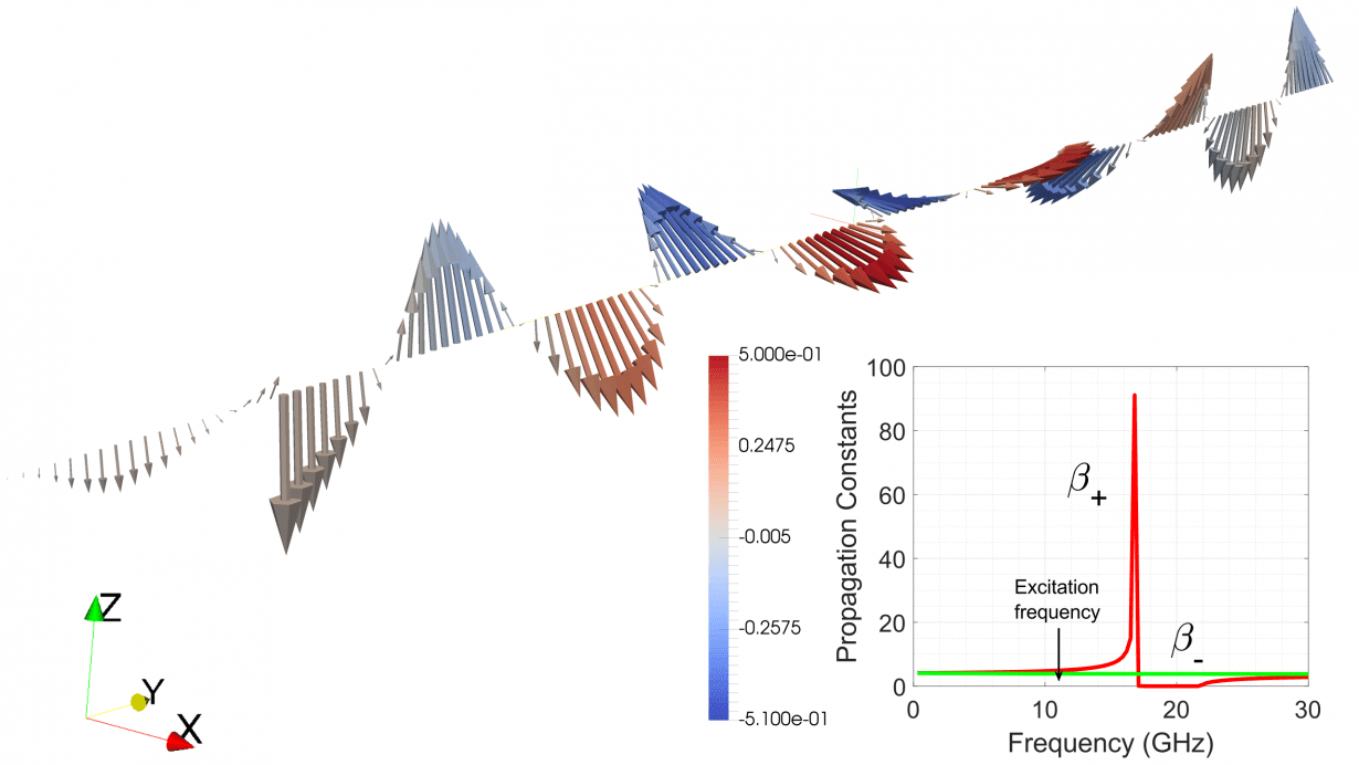
Fig. 2. Electric field vector as function of propagation distance $y$ for excitation frequency of $11$ GHz (and other parameters described above). The field is linearly polarised but rotates with a constant phase according to equations 1 & 2. The inset shows the dependence of propagation constants $\beta _+$ and $\beta _-$ as function of the frequency.

Figure 2 demonstrate the rotation of the vector $E_z$ as a function of propagation distance $y$ . The wave is initially linearly polarised in $z$ , but changes its polarisation with a constant phase $\phi$ along the propagation direction. It should be noted that the excitation frequency in this case is set much below the resonance condition ( $f_H = 16.8$ GHz, at $H = 6$ kOe), so the difference $\beta _+ - \beta _-$ is not significant (see figure #, inset) and the rotation of polarisation is not significant, keeping the electric vector linearly polarised within the cycles. However if the damping parameter is increased or the excitation frequency becomes close to resonance, the RHCP mode becomes damped leading to larger ellipticity and eventually only the LHCP mode remaining with circular polarisation (see figure 3).

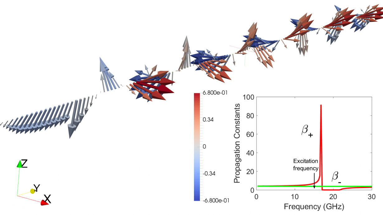
Fig. 3. Electric field vector as function of propagation distance $y$ for excitation frequency of $15$ GHz. The field vectors are not aligned within the cycle and rotate significantly because the of the larger difference between propagation constants $\beta _+$ and $\beta _-$ .

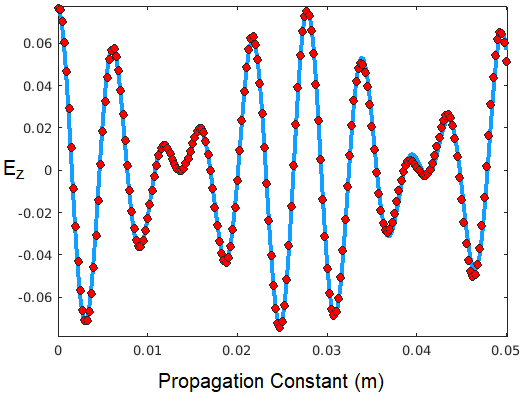
Fig. 4. Electric field intensity $E _z$ as function of propagation distance $y$ as calculated using MaxLLG (red dots) and analytically derived using equation 1.

Figure 4 shows a comparison between the solution produced by MaxLLG solver (red dots) and the analytical solution calculated with equation 1. It is evident that within the first cycles of oscillations along the propagation direction the match is nearly ideal, indicating the validity of the modelling approach as well as the precision of the numerical solution. However the further away from the excitation centre the solutions deviate as the numerical solution is affected by the transient effects and the damping both of which are dependent of the frequency and the damping parameter alpha as discussed above.

[1] Pozar, David M. Microwave Engineering. Hoboken, NJ :Wiley, 2012.

Faraday rotation

You May Also Like

Dispersion characteristics for a magnetostatic wave in tangentially magnetized medium placed inside a parallel plate waveguide

Dispersion characteristics for a magnetostatic wave in unbounded medium

Leave a comment Cancel reply