Propagation in a waveguide loaded with ferrite

One of the standard problems in microwave electronics is propagation of electromagnetic waves in waveguide systems. For waves in the range of ~1- 50 GHz this can be achieved by means of rectangular waveguides, capable of supporting TEM modes. This range of frequencies is also convenient for using ferrites, as it spans over their resonance frequencies which can also be tuned by a practically accessible magnetic field (e.g. by means of permanent magnets). In particular, ferrites are essential in a number of devices, such as isolators and circulators, in which the directionality of the wave propagation is being controlled. This is possible owing to the non-reciprocity effect exhibited by ferrites. Here we demonstrate this effect on an example of a rectangular waveguide partially loaded with ferrite. The schematics of the particular geometry is given on figure 1b. A ferrite slab of thickness d and height h is inserted inside the waveguide at a distance l from one of its walls. The length of both the waveguide and the ferrite slab are assumed to be much larger than the other dimensions. The ferrite slab is fully saturated by applied magnetic field $H$ in the direction of the shorter dimension of the waveguide (parallel to the $E$ field lines) and the propagation of the travelling waves along the waveguide are examined. Here we skip the full description of this problem, which can be found in a number of textbooks on the subject (e.g. [1,2]), but show the general solution describing the steady states can be given by the following equations:

(1) $\begin{equation*} $E_y = \left\{ \begin{array}{ll} \hspace{20mm} A \sin k_a x & \text{for} \hspace{3mm} 0 < x < c \\ B \sin k_f (x - c) + C \sin k_f (c + t - x) & \text{for} \hspace{3mm} c < x < c + t \\ \hspace{15mm} D \sin k_a (a - x) & \text{for} \hspace{3mm} c + t < x < a} \end{array} \right.$ \end{equation*}$

where $k_a = \sqrt{k_0 ^2 - \beta^2}$ and $k_f = \sqrt{\omega^2 \mu_e \epsilon - \beta^2}$ are the cut-off wave numbers for the waves propagating in free space and ferrite. In the latter, $\mu_e = (\mu^2 - \kappa)/ \mu$ is an ‘effective’ permeability, which provides the relation between the propagation constant and the magnetic parameters of the ferrite. A similar set of equations can be derived for the magnetic field $H_x$ , which will include the same scaling coefficients $A,B,C$ and $D$ . Matching both fields at the air/ferrite interfaces allows us to find all four coefficients and thus derive the field profiles for any given parameters of the system. The same equations can be also used to derive the propagation constant $\beta$ . In fact, there are two distinctive solutions, corresponding to either negative or positive value of $\kappa$ , which determine the field profiles depending on either the direction of the wave propagation or the orientation (positive or negative) of the magnetisation vector. Figure 1 shows the profiles (the largest amplitude) of the electric field $E_y$ derived for the two cases. The simulation results, red and yellow dotted lines, are given for the different direction of magnetisation and the bias field $H_0$ , parallel and antiparallel to y-axis. The blue and red lines are the corresponding solutions obtained from equations 1. The ferrite slab in this example is placed in the middle of the wave guide and fills the whole length of the simulation volume. The waveguide is open-ended and the wave is generated at one (top) end and propagates in both directions. As can be seen in the figure, depending on the orientation of the magnetisation the electric field is ‘displaced’ from one or another side of the ferrite.

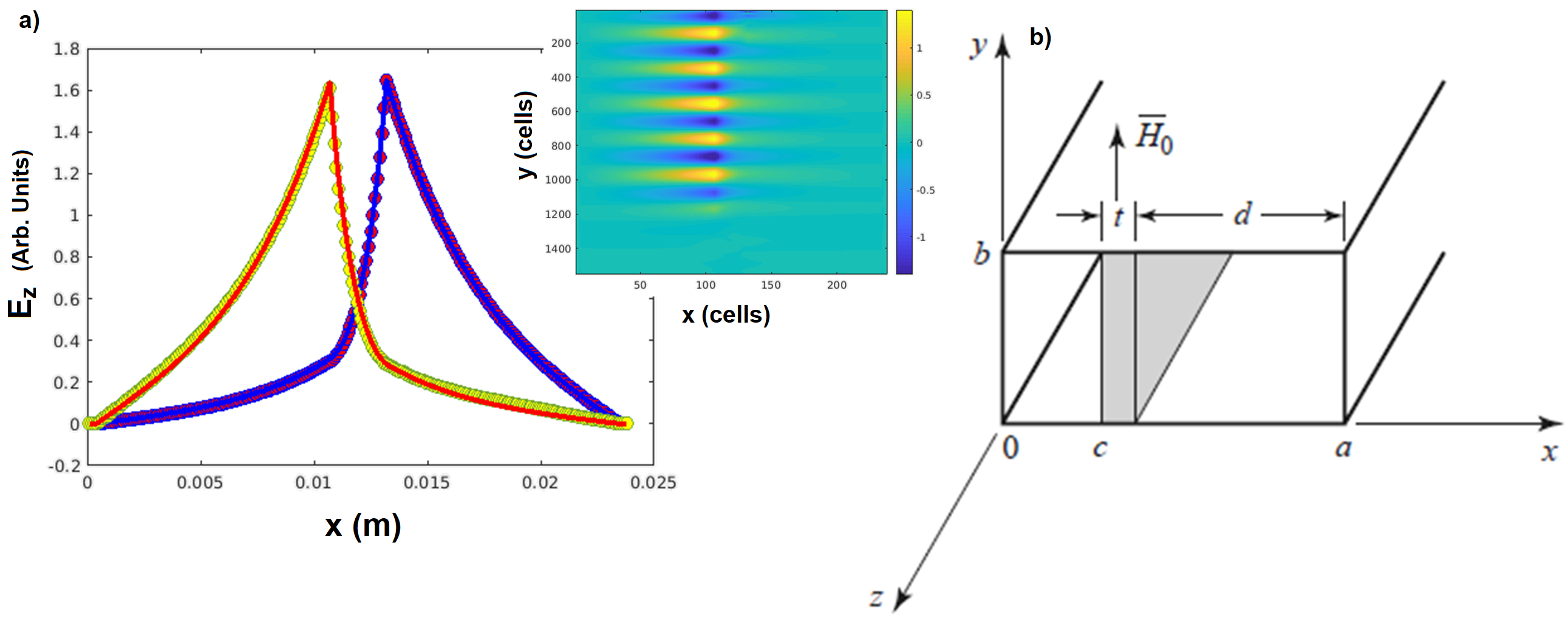
Figure 1. Non-reciprocity effect in the waveguide loaded with a ferrite slab. a) Profile of the electric field $E_z$ for two orientations of the field $H_0$ , or (equivalently) the two orientations of propagation (along – z and +z). Dots – result obtained by MaxLLG solver, Lines – exact solution of equation 1, with the same geometric and material parameters. Inset shows the full intensity map inside the waveguide for the case of negative field. The dash line shows the position where the 2D profile was extracted. b) The geometry of the waveguide and the positioning of the slab.

As in the Faraday rotation case the propagation of the wave inside the ferrite slab very much depends on the parameters of the magnetisation and the magnetic field. In particular if the frequency falls in the region of $\omega_H < \omega < \omega_H + \omega_M$ , as is the case here, the RHCP mode is purely evanescent and the overall propagation in the waveguide is obstructed because of the ‘near-resonance’ conditions. Furthermore, here we have also chosen the conditions when the propagation constant $\beta$ is greater than $k_0$ , so both cut-off wave numbers are purely imaginary and the field profiles, in both ferrite and free space areas, are described by hyperbolic functions [Pozar].

As demonstrated here the results of the simulation are generally in good agreement with the theoretical description. Some discrepancy however can still be observed. In order to obtain the wave pattern some time (associated with the damping constant) has to evolve before the oscillations are stationary. Given the limited dimensions of the waveguide, this time is sufficient for some of the reflected signal to interact with the upcoming wave. This is particularly seen towards the end of the waveguide.

Field displacement isolators.

The non-reciprocity effect has found application in a number of microwave devices, including isolators. The main principle of an isolator is to allow propagation of waves in one direction, but suppress in to the other. The use of isolators is very common in RF circuits, particularly in the cases with parasitic reflections. One possible design of an isolator using the field displacement effect (considered above) is by putting a ferrite slab, as shown in figure 1b, towards one side of the wave-guide, so that the separation is significantly smaller than the width of the guide (typically $\approx 0.05$ m). This is chosen with the aim to obtain the difference in the cut-off propagation constants in forward and reverse orientations. Here we consider an example (considered analytically in [Pozar]), to demonstrate the effect using MaxLLG software. Following the proposed solution we chose the following set of parameters: $c = 19.8$ mm, $t = 2.5$ mm, $a = 23$ mm, $b =12$ mm and $d = a-c-t$ [*]. Applied field $\mu_0 H_0$ and magnetisation $\mu_0 M_s$ will be directed along y axis, with the values of $0.3$ T and $0.12$ T.

0.12 T. Figure 2 shows the plots of electric field intensity $E_y$ in the waveguide at a certain point of time after activation of the signal. The activation is in the plane $xy$ at the beginning of the waveguide, and is achieved with a continuous sine wave polarised in the $y$ direction. As in the example the frequency of oscillation is set to $11$ GHz.

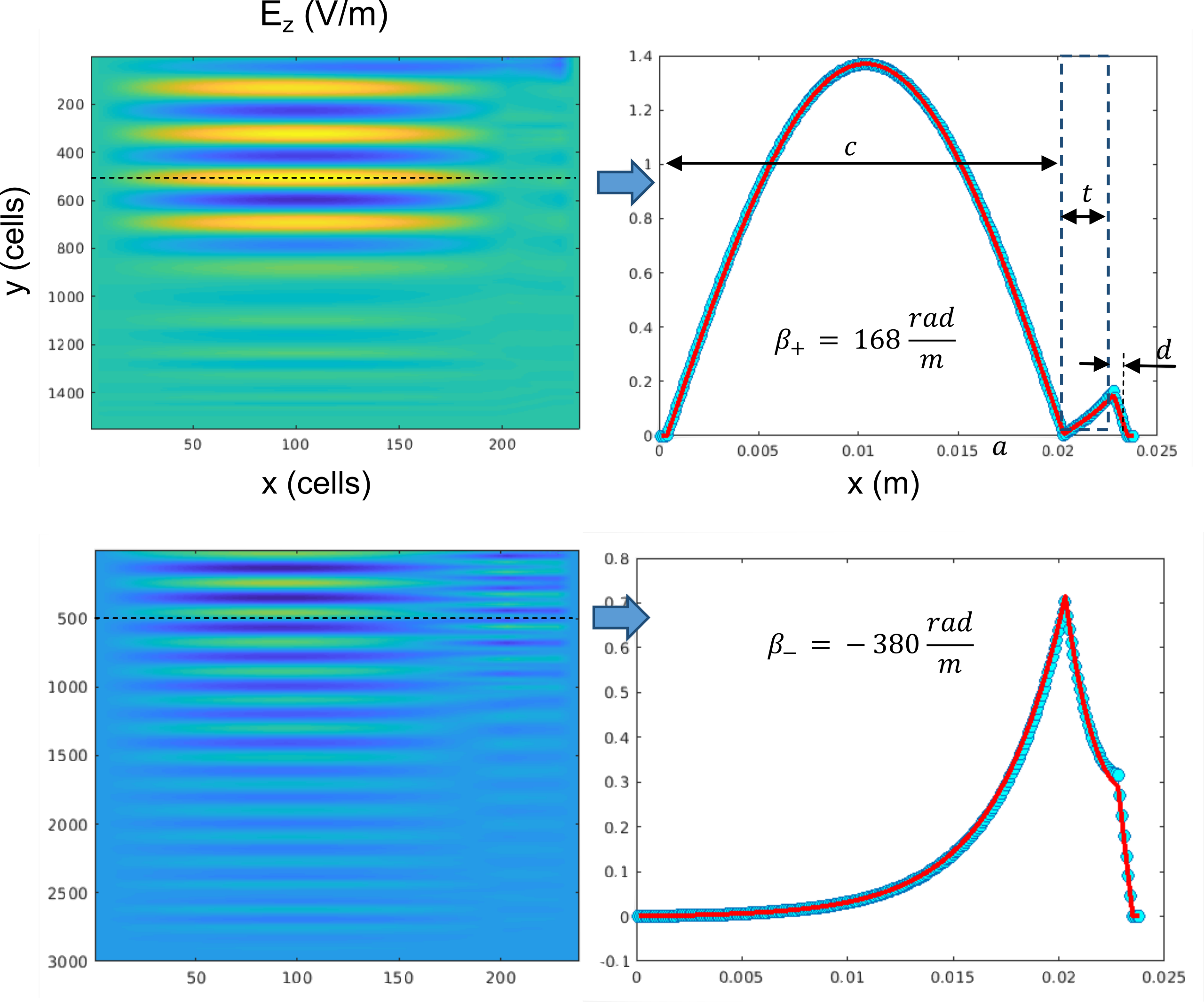
Figure 2. Field displacement isolator. a) Intensity and profile of the electric field $Ez$ for positive value of the applied field ( $\beta_{+} = 168 \dfrac{rad}{m}$ ). b) Intensity and profile of the electric field $E_z$ for negative value of the applied field ( $\beta_{-} = -380 \dfrac{rad}{m}$ ). Dots – result obtained by MaxLLG solver, Lines – exact solution of equation 1, with the same geometric and material parameters. Dashed lines show the position of the profile cut. Dashed square in a) shows the position of the ferrite slab.

The profile of the intensity is taken along the dashed lines, and as in the case of figure 1 it is matched by the analytical expressions obtained from the equation 1. As we can see, in this case there are two distinctive solutions for field (and magnetisation) oriented in opposite directions. In the first example (a), the value of the propagation constant $\beta$ is lower than $k_0$ leading to a real solution. Moreover, the position of the slab is chosen precisely to form a zero on the inner side of the ferrite slab, by satisfying the condition $k_a d = \pi$ In this scenario, the wave propagates without a loss. When changing the direction of the wave propagation on opposite, or equivalently changing the orientation of the field (and thus magnetisation), as shown in example (b), the propagation constant becomes higher than $k_0$ , thus leading to a hyperbolic solution and greater propagation loss.

It should be noted, in this case the solution of equation 3 gives several values of constant $\beta$ for this direction of propagation, as can be seen in figure 3.

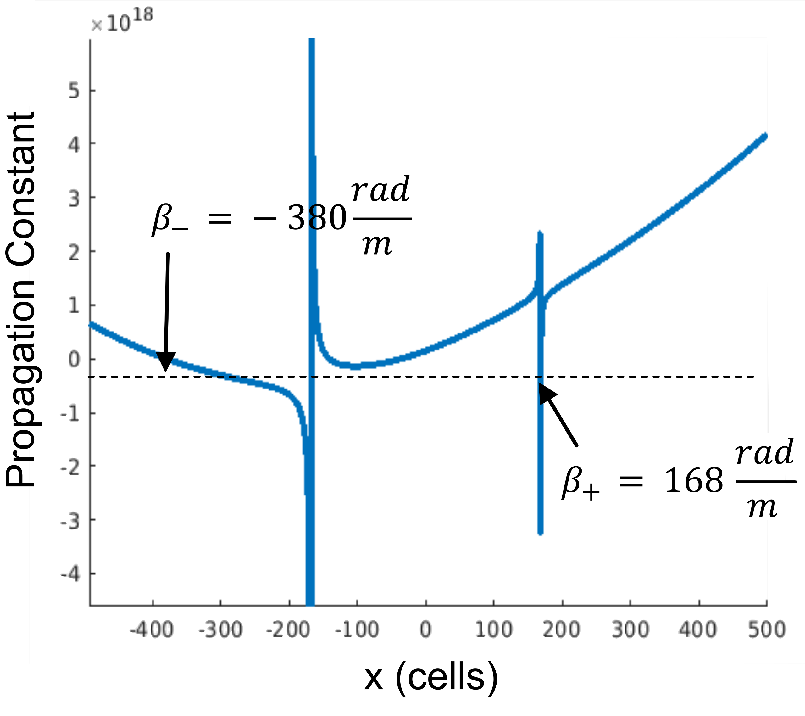
Figure 3. Numerical solution for propagation constant (for the field displacement isolator with the above parameters) . Cross-section of the line with 0 (dashed line) indicate the values of $\beta$ as solutions of equation 1 [Pozar]. Positive branch has one solution $\beta_{+} = 168 \dfrac{rad}{m}$ (figure 2a). Negative branch has several cross-sections, leading to several modes mixed. The dominating mode in the ferrite slab has a propagation constant $\beta_{-} = -380 \dfrac{rad}{m}$ [Pozar].

This leads to the fact that the total wave-form is a mixture of three modes of different amplitudes. This is why the wavelength in free air and the ferrite in the waveguide is different. The smaller propagation constants dominate in the former part. However when measuring the profile in the zero nodes, the profile matches very well the solution in the ferrite, dominated by the wave with the higher value propagation constant (as seen in figure 2b).

[1] Pozar, David M. Microwave Engineering. Hoboken, NJ :Wiley, 2012.

[2] Gurevich, A.G. and Melkov, G.A. Magnetization Oscillations and Waves, Boca Raton :CRC Press, 1996.

[*]… here we use similar arrangements to the example in Pozar’s [1] with the only difference that the slab is displaced to the other side of the waveguide wall. This shows that the solution is still symmetrically the same but changing the sign of the propagation constant.

Propagation in a waveguide loaded with ferrite

You May Also Like

Faraday rotation

Dispersion characteristics for a magnetostatic wave in tangentially magnetized medium placed inside a parallel plate waveguide

Leave a comment Cancel reply